This guide is based on https://tensorflow.rstudio.com/tutorials/beginners/ For a slightly more in-depth manual, consult the original.
install.packages(c("tensorflow", "readmnist"))
library(tensorflow)
Unless you already have installed tensorflow, use the tensorflow package to automatically install tensorflow:
install_tensorflow()
When asked, accept the Miniconda installation variant:
No non-system installation of Python could be found.
Would you like to download and install Miniconda?
Miniconda is an open source environment management system for Python.
See https://docs.conda.io/en/latest/miniconda.html for more details.

Would you like to install Miniconda? [Y/n]:
The tensorflow package needs to be reloaded after the installation of tensorflow
library(tensorflow)
tf$constant("Hello Tensorflow")
install.packages("keras")
library(keras)
The keras package includes a function to download the mnist dataset
mnist <- dataset_mnist()
The mnist data set contains 70.000 gray scale images, see http://yann.lecun.com/exdb/mnist/ for more information. Each pixel (or cell) in each image is a value between 0 and 255, the larger the value, the darker the level of gray. In order for tensorflow to work with the data, it has to be scaled down from the range 0-255 to the range 0-1, so that the maximum value is 1, not 255.
To scale down the data to the target range, divide the data with 255
mnist$train$x <- mnist$train$x/255
mnist$test$x <- mnist$test$x/255
To visualise an element in the mnist training data set, first create the following function.
my.plot <- function(index){
  image(1:28, 1:28, t(apply(mnist$train$x[index,,], 2, rev)),
  col = gray((255:0)/255), main = mnist$train$y[index], xlab = "",
  ylab = "", xaxt = "n", yaxt = "n")
}
Secondly, apply the function with the index of the element you want to visualize, e.g. to visualise the 19th element, call the function like this:
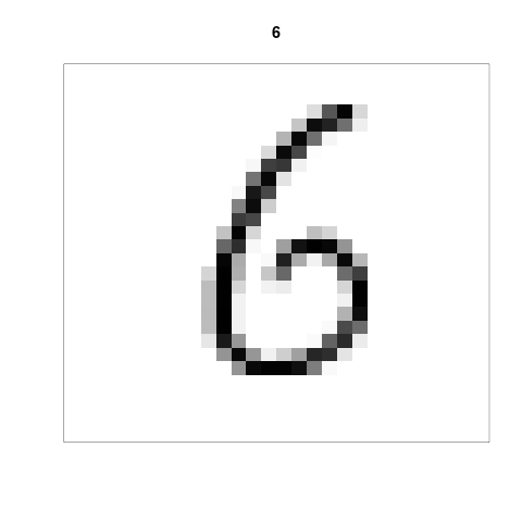
my.plot(19)
which will create the following plot:
The title of the plot indicates the correct classification.
Here we define the structure and the size of the neural network. The input is a an image of 28 by 28 pixels, i.e. each image is a grid of 28 by 28 cells, and each cell contains a color value, the higher the value the darker the gray color in that cell.
model <- keras_model_sequential() %>%
  layer_flatten(input_shape = c(28, 28)) %>%
  layer_dense(units = 128, activation = "relu") %>%
  layer_dropout(0.2) %>%
  layer_dense(10, activation = "softmax")
model %>%
  compile(
    loss = "sparse_categorical_crossentropy",
    optimizer = "adam",
    metrics = "accuracy"
  )
We usually say that we fit the model to data, but in machine learning you often hear that you "train the model". In the keras package, the method we apply to the model is called "fit", and it uses the training data as input.
model %>%
  fit(
    x = mnist$train$x, y = mnist$train$y,
    epochs = 5,
    validation_split = 0.3,
    verbose = 2
  )
Epoch 1/5
1313/1313 - 4s - loss: 0.3427 - accuracy: 0.9012 - val_loss: 0.1882 - val_accuracy: 0.9456 - 4s/epoch - 3ms/step
Epoch 2/5
1313/1313 - 3s - loss: 0.1665 - accuracy: 0.9515 - val_loss: 0.1422 - val_accuracy: 0.9589 - 3s/epoch - 3ms/step
Epoch 3/5
1313/1313 - 3s - loss: 0.1250 - accuracy: 0.9627 - val_loss: 0.1165 - val_accuracy: 0.9656 - 3s/epoch - 2ms/step
Epoch 4/5
1313/1313 - 3s - loss: 0.1010 - accuracy: 0.9695 - val_loss: 0.1073 - val_accuracy: 0.9678 - 3s/epoch - 2ms/step
Epoch 5/5
1313/1313 - 3s - loss: 0.0863 - accuracy: 0.9730 - val_loss: 0.0992 - val_accuracy: 0.9706 - 3s/epoch - 3ms/step
In about 15 seconds the model has trained all its over 100.000 parameters, using a data set consisting of 70% of the full training data set, the remaining 30% of the training data was used to evaluate the model fit.
val_accuracy says how well the model performs on the 30% data set aside for evaluation, which is called the "validation" set.
The predictions come in form of a probability distribution for each possible outcome
predictions <- predict(model, mnist$train$x)
predictions now holds all the predicted probabilities for all possible outcomes from all elements from the training data set. To print out the predicted probabilities for the first element, use
round(predictions[1, ], 2)
[1] 0.00 0.00 0.00 0.15 0.00 0.85 0.00 0.00 0.00 0.00
These probabilities implictly corresponds to these outcomes
[1] 0 1 2 3 4 5 6 7 8 9
To get the most likely classification for the element with index k, define a function
my.one.hot <- function(k) {
which(predictions[k, ] == max(predictions[k, ])) - 1
}
my.one.hot(1)
[1] 5
And for the 19th element, use
my.one.hot(19)
[1] 6
We can now modify the plot function to include the most likely classification in the title by modifying the argument "main".
my.plot <- function(index){
  image(1:28, 1:28, t(apply(mnist$train$x[index,,], 2, rev)),
  col = gray((255:0)/255), main = paste("correct:", mnist$train$y[index],
  "prediction:", my.one.hot(index)), xlab = "", ylab = "", xaxt = "n", yaxt = "n")
}
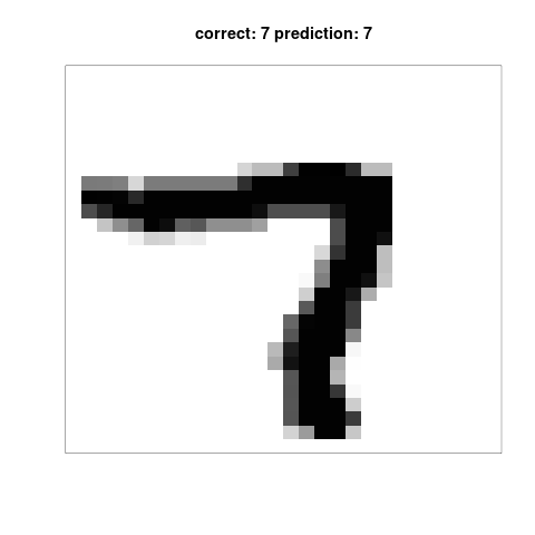
Now the plot includes both the correct answer and the answer given by the neural network model, this code
my.plot(19)
produces this plot:

So far, we have only evaluated the predictions, ie classifications, on data that in some way or another was used in the training process, either as training data, in which case the model as speficially adjusted to make predictions as close as the correct answers as possible) or as validation data, in which case the data could have been used to select between competing models (model selection was AFAIK not used here though).
The real test is to let the model predict on data never used in any way in the training process. To apply model on unseen data, use the evaluate() method, i.e. function, of the model object.
model %>%
  evaluate(mnist$test$x, mnist$test$y, verbose = 0)
That the output of the model is a probability distribution, i.e. a list of probabilities, is a bit inconvenient when we only want a single answer, but it is helpful when we want to quantify the certainty of each prediction, since the variance of the probability distribution is highest for a one-hot encoding.
To calculate the variance for each "row" in the predictions object, use this code:
certainties <- apply(predictions, 1, var)
The certainty is highest when all the probability is on a single outcome, and here is how the output looks for the row with least certainty:
round(predictions[which(certainties == max(certainties)),], 4)
[1] 0 0 0 0 0 0 0 1 0 0
Compare that to the outcome where the certainty is highest (and conversely, the variance is the lowest):
round(predictions[which(certainties == min(certainties)),], 4)
[1] 0.0796 0.0001 0.0389 0.1587 0.1709 0.0446 0.2680 0.0013 0.1267 0.1110
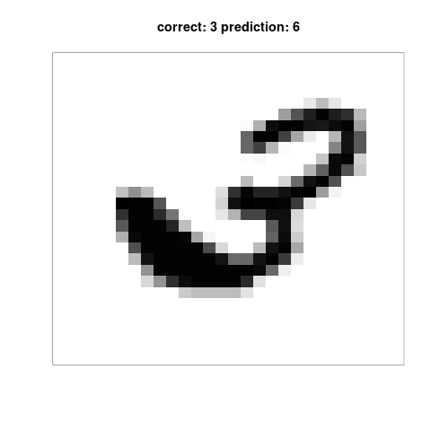
We can also inspect the "easiest-to-classify"-digit and the "hardest-to-classify"-digit, along with their classifications.
my.plot(which(certainties == max(certainties)))
my.plot(which(certainties == min(certainties)))
I did not find it obvious why these particular digits was easy or hard, so to ensure that the method was sound, I plot the top 9 easiest and the top 9 hardest digits.
par(mfcol=c(3, 3)) ## arrange 9 graphs in a 3 by 3 grid figure
for(i in tail(order(certainties), 9)){
  ## i holds the index of the 9 most certain classifications
  my.plot(i)
}
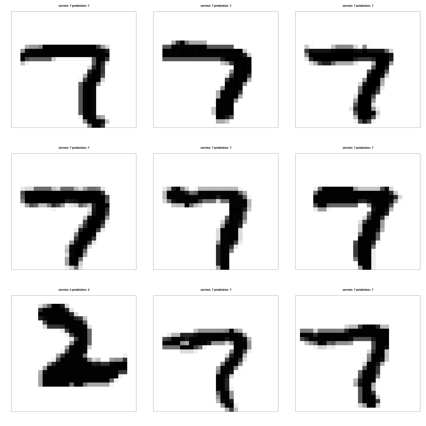
Below follows the top 9 hardest elements to classify, according to the model itself.
Apparantly, 7 is a digit easy to recognise.
par(mfcol=c(3, 3))
for(i in head(order(certainties), 9)){
  my.plot(i)
}

![[Valid RSS]](valid-rss-rogers.png "Validate my RSS feed")

