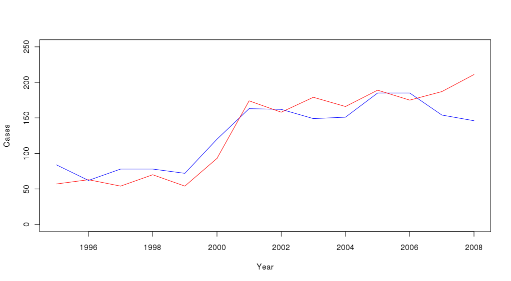
Take a look at the following graph:
The blue line represents the number av male suspects for a certain crime, the red line represents the number of female suspects for the same crime.
To me, it seems that as if the blue curve generally was above the red line up to the year 2000, and after 2000, the red curve (the number of female suspects) is generally above the blue line. The hypothesis that I would like to test is that the at some point during the year 2000 the order of the number of male and female suspects is reversed, and that this not simply a result of random variation in the yearly number of suspects.
Group the years in two groups 1995-2000 in one group and 2001-2008 in the other group. Make a crosstable, and use a chi² test.
matrix(c(sum(Women[Year < 2001]), sum(Men[Year < 2001]), sum(Women[Year > 2000]), sum(Men[Year > 2000])), nrow = 2)
     [,1] [,2]
[1,]  391 1439
[2,]  494 1295
And the test
chisq.test(matrix(c(sum(Women[Year < 2001]), sum(Men[Year < 2001]), sum(Women[Year > 2000]), sum(Men[Year > 2000])), nrow = 2))

	Pearson's Chi-squared test with Yates' continuity correction

data:  matrix(c(sum(Women[Year < 2001]), sum(Women[Year > 2000]), sum(Men[Year < 2001]), sum(Men[Year > 2000])), nrow = 2)
X-squared = 18.7734, df = 1, p-value = 1.472e-05
Or, if you prefer simulations, let's create p out of 1.000.000 simulations:
chisq.test(matrix(c(sum(Women[Year < 2001]), sum(Women[Year > 2000]), sum(Men[Year < 2001]), sum(Men[Year > 2000])), nrow = 2),
   simulate.p.value = TRUE, B = 1000000)

	Pearson's Chi-squared test with simulated p-value (based on 1e+06
	replicates)

data:  matrix(c(sum(Women[Year < 2001]), sum(Women[Year > 2000]), sum(Men[Year < 2001]), sum(Men[Year > 2000])), nrow = 2)
X-squared = 19.11, df = NA, p-value = 1.3e-05
So there was indeed a change in the relative numbers of female vs male suspects of this crime in the year 2000.
Let's say you'd like a function that for each year gives you the p-value for the existance of a reverse taking place between 2000 and 2001. Such a function would report larger p-values for low number of years and 1.3e-05 for 8 years, which is covering the whole period. The line-breaks in the examples are optional.
sapply(1:8, function (x) {chisq.test(matrix(c(sum(Women[Year < 2001 & Year >= 2001-x]),
   sum(Men[Year < 2001 & Year >= 2001-x]), sum(Women[Year > 2000 & Year <= 2000+x]),
   sum(Men[Year > 2000 & Year <= 2000+x])), nrow = 2))$p.value})
plot(1:8, sapply(1:8, function (x) {chisq.test(matrix(c(sum(Women[Year < 2001 & Year >= 2001-x]),
   sum(Men[Year < 2001 & Year >= 2001-x]), sum(Women[Year > 2000 & Year <= 2000+x]),
   sum(Men[Year > 2000 & Year <= 2000+x])), nrow = 2))$p.value}),
  type = "l", xlab = "Years around 2000-2001 included", ylab = "p",
     main = "p as a function of included number of years from the break in 2000-2001")
And you might want a line showing where the conventional limit for significance comes in.
lines(x=1:8, y=rep(0.05,8), col ="red")
 *
*
And, if you wonder, the crime at stake is when one of the parents removes the child from the other parent (legal guardian), often in cases of joint custody, but also happens when one parent loses custody to the other parent but refuses to accept the court's decision. 1998 there was an important change in the law, the courts where given the power to rule joint custody even if that was not accepted by both parents. The dramatic rise in the total number of cases between 1999 and 2001 is an delayed effect of that change in legislation, and accompanying that increase in number of cases, more mothers (red line) rather than fathers (blue line) now find the courts decisions unacceptable.
Do you dislike repetion of expressions? Prefer using variables instead?
OK, here is the same code but enhanced for your preferences, using ct as a variable containing the crosstable, and pt a vector of p-values.
ct <- matrix(c(sum(Women[Year < 2001]), sum(Men[Year < 2001]), sum(Women[Year > 2000]), sum(Men[Year > 2000])), nrow = 2)
ct
chisq.test(ct)
chisq.test(ct, simulate.p.value = TRUE, B = 1000000)
pt <- sapply(1:8, function (x) {chisq.test(matrix(c(sum(Women[Year < 2001 & Year >= 2001-x]),
   sum(Men[Year < 2001 & Year >= 2001-x]), sum(Women[Year > 2000 & Year <= 2000+x]),
   sum(Men[Year > 2000 & Year <= 2000+x])), nrow = 2))$p.value})
pt
plot(pt, type = "l", xlab = "Years around 2000-2001 included", ylab = "p",
     main = "p as function of included number of years from the break in 2000-2001")
lines(x=1:8, y=rep(0.05,8), col ="red")
Or, do you consider it ugly to specify the matrix "manually" two times rather then defining a function that could be used both to create the first matrix ct and the matrix used to create pt? Then a function for that would look like this:
my.matrix <- function (x) {
   matrix(c(sum(Women[Year < 2001 & Year >= 2001-x]),
   sum(Men[Year < 2001 & Year >= 2001-x]), sum(Women[Year > 2000 & Year <= 2000+x]),
   sum(Men[Year > 2000 & Year <= 2000+x])), nrow = 2) }
ct <- my.matrix(8)
ct
chisq.test(ct)
chisq.test(ct, simulate.p.value = TRUE, B = 1000000)
pt <- sapply(1:8, function (x) {chisq.test(my.matrix(x))$p.value})
pt
plot(pt, type = "l", xlab = "Years around 2000-2001 included", ylab = "p",
     main = "p as a function of included number of years from the break in 2000-2001")
lines(x=1:8, y=rep(0.05,8), col ="red")
While a visual inspection suggests that the break occurs between 2000 and 2001 - in parallell with the dramatic increase of the overall number of cases - it might be reassuring if a statistical analysis too would indicate that particular point in time as the break.
The function my.matrix could be generalised to split groups on any given year, given as a second argument. And then that function could be used to find the year that maximises the differences between "before" and "after" in regard to fathers and mothers relative numbers of crimes.
y can be in the range 1996 to 2008
my.matrix <- function (x, y) {
   matrix(c(sum(Women[Year < y & Year >= y-x]),
   sum(Men[Year < y & Year >= y-x]), sum(Women[Year > y-1 & Year <= y-1+x]),
   sum(Men[Year > y-1 & Year <= y-1+x])), nrow = 2) }
Let p be a function of year y. Create a list of p-values by applying the function for each year between 1996 and 2008. Sort the list and print the year and p-value at the top.
years <- 1996:2008
pt <- sapply(years, function (y) {chisq.test(my.matrix(8, y))$p.value})
names(pt) <- years
head(sort(pt), 1)
   2001
1.5e-05
Nice to know that R agrees on where to make the split. If you still want a visual display of all break-points that creates a p-value less than 0.05:
sig.pt <- pt[pt < 0.05]
plot(names(sig.pt), sig.pt, xlab = "Year to split on", ylab = "p-value")

So, the analysis points to between 2001 and 2000, the break seems to have taken place then, since splitting the period in groups at that point creates the smallest p-value for the hypothesis that there is a different proportion of suspect mothers and fathers before and after that year. A p-value of 1.5e-05 means that the probability of having the distributions of female/male suspects before and after the break by chance - meaning there is no real break - is 1 in 66 667. However, splitting on 2001-2002 or 2002-2003 gives almost as low p-values as splitting on 2000-2001.
![[Valid RSS]](valid-rss-rogers.png "Validate my RSS feed")

