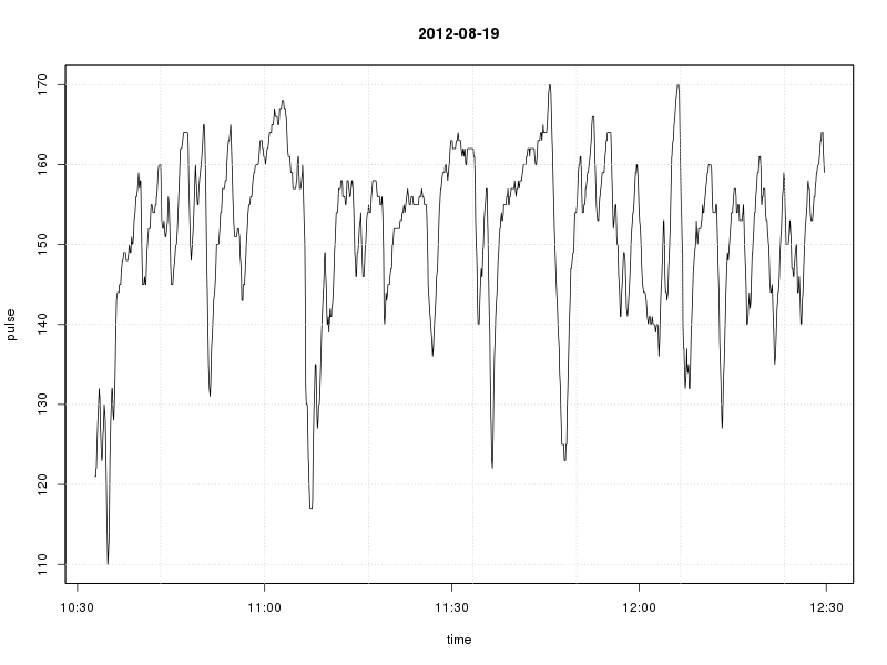
Analysing data from physical training sessions

Two years ago, I bought a Garmin Forerunner 305 to records pulse and location during my training sessions. pytrainer does a good job graphing sporting excursions such as running or cycling sessions, but with a little bit of R code, you can do your own analysis and graphing. Most of the code needed is already written and compiled into nice high-level libraries for R, eg the plotKML, sp, zoo, and XML packages.

Instructions for installing plotKML,

Read data from the GPS device, and reading the xml data into R

There are two ways to get the data from the device, each has its own package

gpsbabel is convenient to use, but it does not extract the total distance which garmin fore runner 305 records at each point. While latitude and longitude plus elevation can be used to derive this distance, garmin-forerunner-tools provides this data directly from the device. The only drawback of garmin-forerunner-tools is that the procedure needed to get data from the device into R has an extra step.

Using gpsbabel

Instructions for installing gpsbabel

system("sudo gpsbabel -t -i garmin -f usb: -o gpx,garminextensions -F ~/my.gpx")
library(XML)
my.xml.tree <- xmlParse(file="my.gpx")

The alternative is using the commands in the package garmin-forerunner-tools.

Using garmin-forerunner-tools

my.dir <- system("mktemp -d", intern = TRUE)
setwd(my.dir)
system("sudo garmin_save_runs")
system("sudo chown -R hans:hans .")
my.files <- list.files(pattern=".gmn", recursive=T)
my.xml.data <- system(paste("garmin_dump", my.files[6]), intern = TRUE) ## Reading only the session in file number 6.
my.xml.tree <- htmlTreeParse(my.xml.data)
r <- xmlRoot(my.xml.tree)[[1]]
## xmlattrs(xmlchildren(r)[[2]])

Plot heartrate over time

my.activity <- xmlAttrs(xmlChildren(r)[[1]])[['sport']]
my.session <- xmlAttrs(xmlChildren(r)[[1]])[['track']]
my.start.time <- as.POSIXct(xmlAttrs(xmlChildren(r)[[2]])[['start']], format = "%Y-%m-%dT%H:%M:%S")
## duration is in form HH:MM:SS.S
my.duration <- xmlAttrs(xmlChildren(r)[[2]])[['duration']]
## distance is in meters
xmlAttrs(xmlChildren(r)[[2]])[['distance']]

## waypoint data are in nodes named "point"
these <- which(names(sapply(xmlChildren(r), names)) == "point")
## throw away the last waypoint, since it misses most of the variables
these <- these[-length(these)]
my.mat <- matrix(NA, ncol = length(xmlAttrs(xmlChildren(r)[[these[1]]])), nrow = length(these))
##for(i in 1:550){
for(i in these[-length(these)]){
  my.mat[i-(these[1]-1),] <- xmlAttrs(xmlChildren(r)[[i]])
}
my.df <- data.frame(time.stamp = as.POSIXct(my.mat[,2], format = "%Y-%m-%dT%H:%M:%S"), lat = as.numeric(my.mat[,3]), lon = as.numeric(my.mat[,4]), altitude = as.numeric(my.mat[,5]), distance = as.numeric(my.mat[,6]), heart.rate = as.integer(my.mat[,7]))

my.df$dt.time <- c(0, my.df$time.stamp[-1] - my.df$time.stamp[-length(my.df$time.stamp)])
my.df$dt.distance <- c(0, my.df$distance[-1] - my.df$distance[-length(my.df$distance)])
my.df$speed <- c(0, my.df$dt.distance[-1]/my.df$dt.time[-1]) * 3.6

## Absolute time
library(zoo)
my.ts <- zoo(my.df$heart.rate, my.df$time.stamp)
plot(my.ts, xlab = "time", ylab = "pulse", main = as.Date(rownames(as.data.frame(my.ts[1]))))
grid()

## Relative time, custom time labels
my.steps <-  c(0, 3600 * as.numeric(tail(my.df$time.stamp, 1) - head(my.df$time.stamp, 1)) / 4 / 60 * 1:4)
my.hour <- floor(my.steps / 60)
my.minute <- floor(my.steps - 60 * floor(my.steps / 60))
my.lab <- paste(my.hour, formatC(my.minute, flag = "0", width = 2), sep = ":")
plot(y = my.df$heart.rate, my.df$time.stamp - my.df$time.stamp[1], xaxt = "n", ylab = "pulse", xlab = "time", type = "l")
axis(side = 1, at = c(0, 3600 * as.numeric(tail(my.df$time.stamp, 1) - head(my.df$time.stamp, 1)) / 4 * 1:4), labels = my.lab)
grid()

B* Animation

List the named sessions

xpathSApply(my.xml.tree,'//ns:name', xmlValue,
  namespaces = c(ns = "http://www.topografix.com/GPX/1/1"))
[1] "11" "12" "13" "14" "15" "16" "17" "18" "19" "20" "21" "22" "23" "24" "25" "26"
"27" "28" "29" "30" "31" "32

Getting data from a named session

Let's say we wanted to do a time series analysis of heart rate data from the session named "24". For the time serie analysis, we use the package zoo

library(zoo)
my.ts <- zoo(as.numeric(xpathSApply(my.xml.tree,
'//*/ns:name[text()[contains(.,"24")]]//following-sibling::ns:trkseg/*/ns:extensions',
xmlValue, namespaces = c(ns = "http://www.topografix.com/GPX/1/1"))),
             as.POSIXct(strptime(xpathSApply(my.xml.tree,
'//*/ns:name[text()[contains(.,"24")]]//following-sibling::ns:trkseg/ns:trkpt/ns:time',
xmlValue, namespaces = c(ns = "http://www.topografix.com/GPX/1/1")), tz = "GMT",
format = "%Y-%m-%dT%H:%M:%SZ")))

To plot the heart rates over time in this session, we can now simply call plot()

plot(my.ts, xlab = "time", ylab = "pulse", main = as.Date(rownames(as.data.frame(my.ts[1]))))
grid()

Compare two sessions

In order to compare two sessions, the time data in each session must be relative to the starting point of each session - currently the time data are absolute. By substracting the time of the first observation from all observation, we get relative time data.

Eg. Compare session 32 with session 33

my.ts.1 <- zoo(1E11 * as.numeric(xpathSApply(my.xml.tree,
'//*/ns:name[text()="40"]//following-sibling::ns:trkseg/*/ns:extensions',
xmlValue, namespaces = c(ns = "http://www.topografix.com/GPX/1/1"))),
             as.POSIXct(strptime(xpathSApply(my.xml.tree,
'//*/ns:name[text()="40"]//following-sibling::ns:trkseg/ns:trkpt/ns:time',
xmlValue, namespaces = c(ns = "http://www.topografix.com/GPX/1/1")), tz = "GMT",
format = "%Y-%m-%dT%H:%M:%SZ")))
## Save the date
my.title <- as.Date(index(my.ts.1)[1])
## use time differences, not time stamps
index(my.ts.1) <- index(my.ts.1) - index(my.ts.1)[1]
my.ts.2 <- zoo(1E11 * as.numeric(xpathSApply(my.xml.tree,
'//*/ns:name[text()="41"]//following-sibling::ns:trkseg/*/ns:extensions',
xmlValue, namespaces = c(ns = "http://www.topografix.com/GPX/1/1"))),
             as.POSIXct(strptime(xpathSApply(my.xml.tree,
'//*/ns:name[text()="41"]//following-sibling::ns:trkseg/ns:trkpt/ns:time',
xmlValue, namespaces = c(ns = "http://www.topografix.com/GPX/1/1")), tz = "GMT",
format = "%Y-%m-%dT%H:%M:%SZ")))
index(my.ts.2) <- index(my.ts.2) - index(my.ts.2)[1]
my.x.max <- max(c(index(my.ts.1), index(my.ts.2)))
my.y.max <- max(my.ts.1, my.ts.2)
plot(my.ts.1, xlab = "time", ylab = "pulse", main = my.title, xlim = c(0, my.x.max), ylim = c(50, my.y.max))
lines(my.ts.2, lty = 2)

Plot the route using google-earth

library(plotKML)
library(spacetime)
my.df <- data.frame(time = time.stamps <- as.POSIXct(strptime(xpathSApply(my.xml.tree,
'//*/ns:name[text()[contains(.,"24")]]//following-sibling::ns:trkseg/ns:trkpt/ns:time',
xmlValue, namespaces = c(ns = "http://www.topografix.com/GPX/1/1")), tz = "GMT",
format = "%Y-%m-%dT%H:%M:%SZ")))
pos <- t(xpathSApply(my.xml.tree,
'//*/ns:name[text()[contains(.,"24")]]//following-sibling::ns:trkseg/ns:trkpt',
xmlAttrs, namespaces = c(ns = "http://www.topografix.com/GPX/1/1")))
pos.df <- data.frame(lon = as.numeric(pos[ ,2]), lat = as.numeric(pos[ ,1]))
coordinates(my.df) <- pos.df
proj4string(my.df) <- CRS("+proj=longlat +datum=WGS84")
plotKML(my.df, folder.name="/tmp/bar", open.kml = FALSE)
Plotting the first variable on the list
KML file opened for writing...
Writing to KML...
Closing  /tmp/bar.kml
Object written to: /tmp/bar.kml

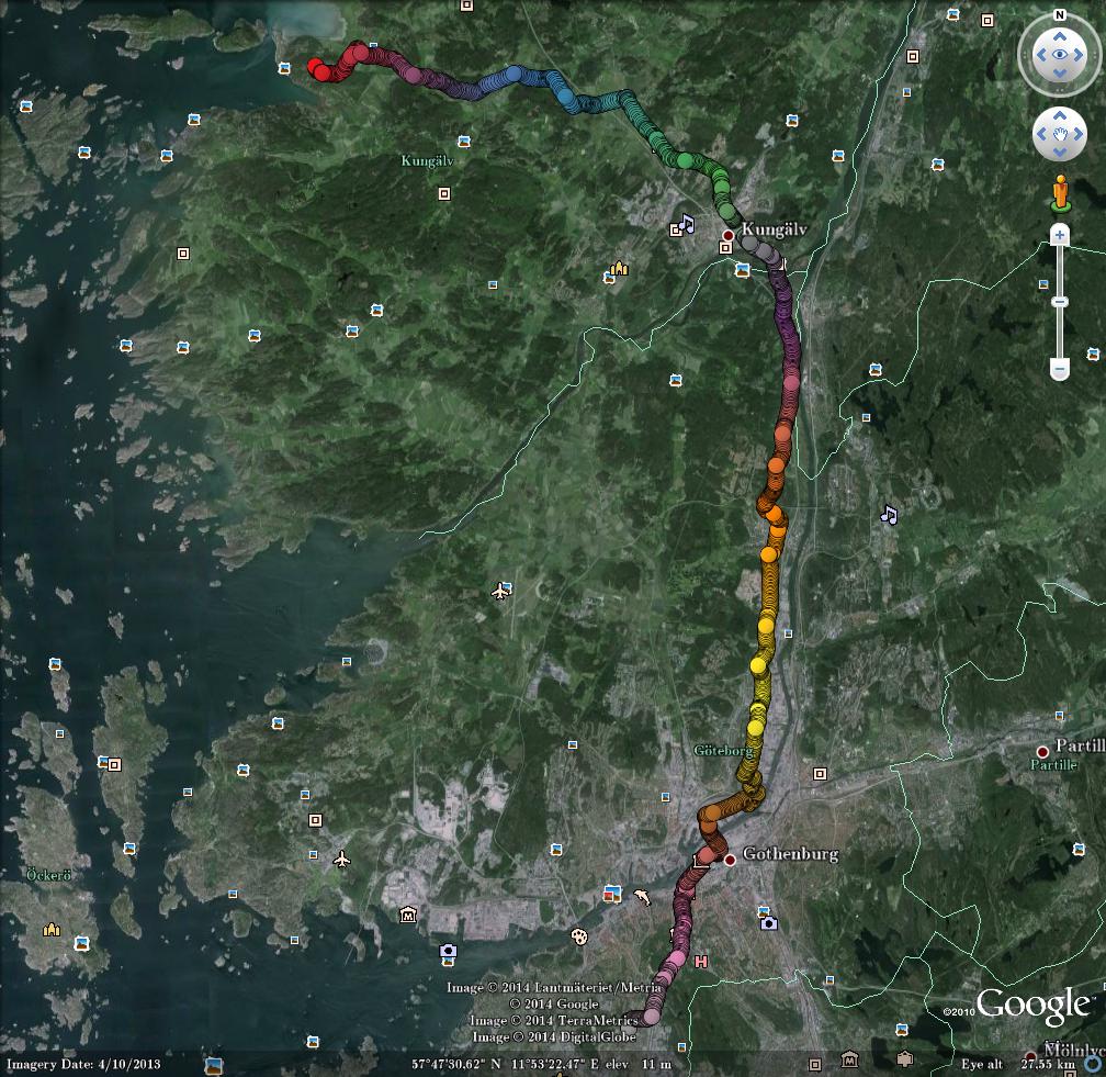
Start google-earth, open /tmp/bar.kml, save as image, and you will get something like this:

Or just share the kml-file for others to open in google-earth.

library(spacetime)
my.gpx <- readGPX("~/my.gpx")
## merge all training sessions into a common data.frame
## This fails unless there are exactly the same numbers of columns in all sessions.
my.df <- data.frame()
for(i in 1:length(my.gpx$tracks)){
  for(j in 1:length(my.gpx$tracks[[i]])){
    if(length(my.gpx$tracks[[i]][[j]]) > 0){
      my.gpx$tracks[[i]][[j]]$session <- i
      print(paste(ncol(my.gpx$tracks[[i]][[j]]), "i:", i, "j:", j))
      my.df <- rbind(my.df, my.gpx$tracks[[i]][[j]])
    }
  }
}

Instructions to install `plotKML` on Debian Wheezy

Make available gdal-config

apt-get install libgdal-dev tk-dev

install plotKML within R

install.packages("plotKML", "fossil")

Uninstall the installed development libraries

To save disk space you may now uninstall the newly installed development libraries. But the runtime library libgdal1 should be kept.

apt-get install libgdal1
apt-get --purge remove libgdal-dev tk-dev
apt-get --purge autoremove

sudo apt-get install googleearth-package
make-google-earth-package
sudo dpkg -i googleearth_6.0.3.2197+0.7.0-1_i386.deb
sudo apt-get -f install
sudo dpkg -i googleearth_6.0.3.2197+0.7.0-1_i386.deb

Instructions for installing gpsbabel

apt-get install gpsbabel

Instructions for installing garmin-forerunner-tools

apt-get install garmin-forerunner-tools

my.ts.1 <- my.ts <- zoo(as.numeric(xpathSApply(my.xml.tree, '//*/ns:name[text()="33"]//following-sibling::ns:trkseg/*/ns:extensions', xmlValue, namespaces = c(ns = "http://www.topografix.com/GPX/1/1"))),

as.POSIXct(strptime(xpathSApply(my.xml.tree, '//*/ns:name[text()="33"]//following-sibling::ns:trkseg/ns:trkpt/ns:time', xmlValue, namespaces = c(ns = "http://www.topografix.com/GPX/1/1")), tz = "GMT", format = "%Y-%m-%dT%H:%M:%SZ"))) Save the date session.1.date <- as.Date(index(my.ts.1)¹) use time differences, not time stamps index(my.ts.1) <- index(my.ts.1) - index(my.ts.1)¹ my.ts.2 <- my.ts <- zoo(as.numeric(xpathSApply(my.xml.tree, '//*/ns:name[text()="34"]//following-sibling::ns:trkseg/*/ns:extensions', xmlValue, namespaces = c(ns = "http://www.topografix.com/GPX/1/1"))), as.POSIXct(strptime(xpathSApply(my.xml.tree, '//*/ns:name[text()="34"]//following-sibling::ns:trkseg/ns:trkpt/ns:time', xmlValue, namespaces = c(ns = "http://www.topografix.com/GPX/1/1")), tz = "GMT", format = "%Y-%m-%dT%H:%M:%SZ"))) session.2.date <- as.Date(index(my.ts.2)¹) index(my.ts.2) <- index(my.ts.2) - index(my.ts.2)¹ my.x.max <- max(c(index(my.ts.1), index(my.ts.2))) my.y.max <- max(my.ts.1, my.ts.2) plot(my.ts.1, xlab = "time (in seconds)", ylab = "pulse", main = "Comparison of training sessions", xlim = c(0, my.x.max), ylim = c(50, my.y.max)) lines(my.ts.2, lty = 2) legend(x = my.x.max / 2.5, y = 60 + (my.y.max - 60) / 2, legend = c(session.1.date, session.2.date), lty = c(1, 2), text.width = strwidth(session.1.date))